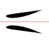
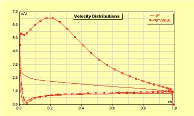
a = 0°
a = -5°
The largest machines of this type were built in the former Soviet Union, though.
Wing in Ground Proximity (WIG) |
From the beginning, JavaFoil had the basic capability to handle multi-element airfoils. This capability was hidden, though. Based on these foundations it was relatively easy (within a few days) to add a ground effect simulation. Internally this option works by creating a mirror image of the current airfoil below the ground, which is assumed to be at y=0. This creates a system of multiple airfoils which is symmetrical about the y=0 plane. The flow around this system can be analyzed using the panel method and the usual boundary layer analysis can be performed to calculate the friction drag.
Note: For highest performance, one would implement such features like ground effect or a cascade option by adapting the calculation of the aerodynamic influence coefficients inside the panel method. Thus one would keep the equation system to be solved at the same size as for a single airfoil. In JavaFoil, the way of actually duplicating the airfoil for the WIG simulation has been chosen. This leads to a more straightforward coding scheme and fits the multi-element option perfectly.
|
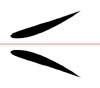
a = 0° |
a = -5° |
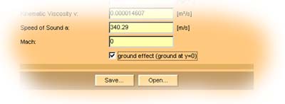
In order to analyze the flow at different angles of attack, the geometry has to be rebuilt for each angle of attack because the geometry of the system must stay symmetrical (see pictures at left). This requires a new panel analysis for each angle of attack, which makes the analysis slower than the plain airfoil analysis. JavaFoil does all this behind the scenes so all you have to do is to toggle the ground effect switch on the Options card. |
|
|
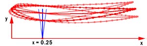
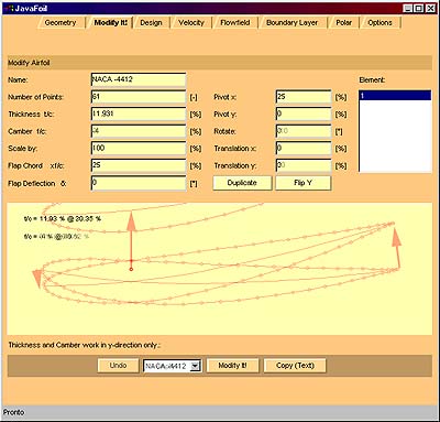
During the WIG simulation the angle of attack of the airfoil is changed by rotating the airfoil around the point (0.25/0). This point is located on the ground as shown at the left. | |
|
|
While the example below shows a downforce application, ground effect can
also be used to increase lift without increasing drag excessively.
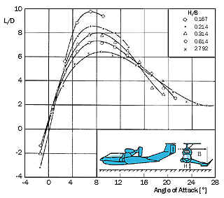
This results in an improved ratio of L/D for lifting applications. Such
devices have been employed in vehicles traveling with reduced power over
flat surfaces, mainly over water. Starting in the 1960s, Alexander Lippisch
was probably one of the first to exploit this phenomenon in his various
ground effect machines. The results of wind tunnel tests for one of his
designs (the X-114) are presented at the left. They show an increase in L/D
from about 6 to 10 for the complete aircraft (tests were conducted at the
German Aerospace Research Center DLR in 1979).
The largest machines of this type were built in the former Soviet Union, though. |
|
An Example: Front Wing of a Race Car |
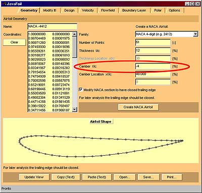
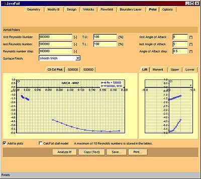
The following example shows, how JavaFoil can be used to analyze the effect of ground proximity on the downforce of an airfoil. Such a condition could occur on the front wing of a race car. As this is only a simple example, the results should not be taken as general. It is clear that an airfoil must be designed and optimized to work efficiently in ground effect. If you want to use this feature in JavaFoil, it is recommended to plan exactly what you want to analyze and which steps you have to perform in order.
Geometry Card |
|
|
 |
Modify Card |
|
|
 |
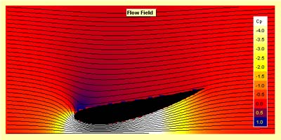
Flow Field Card |
|
Note: for "free flight", the y=0 axis is always located at the center of the graph. |
 |
Options Card |
|
|
 |
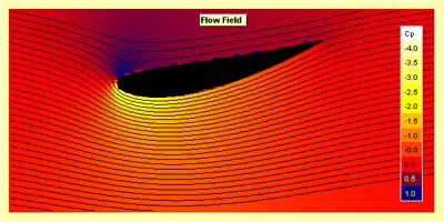
Flow Field Card |
|
Note: with ground effect activated, the y=0 axis is always located at the lower edge of the graph. |
 |
Velocity Distribution Card |
|
|
 |
Polar Card |
|
|
 |
Last modification of this page: 21.05.18
![]()
[Back to Home Page] Suggestions? Corrections? Remarks? e-mail: Martin Hepperle.
Due to the increasing amount of SPAM mail, I have to change this e-Mail address regularly. You will always find the latest version in the footer of all my pages.
It might take some time until you receive an answer
and in some cases you may even receive no answer at all. I apologize for this, but
my spare time is limited. If you have not lost patience, you might want to send
me a copy of your e-mail after a month or so.
This is a privately owned, non-profit page of purely educational purpose.
Any statements may be incorrect and unsuitable for practical usage. I cannot take
any responsibility for actions you perform based on data, assumptions, calculations
etc. taken from this web page.
© 1996-2018 Martin Hepperle
You may use the data given in this document for your personal use. If you use this
document for a publication, you have to cite the source. A publication of a recompilation
of the given material is not allowed, if the resulting product is sold for more
than the production costs.
This document may accidentally refer to trade names and trademarks, which are owned by national or international companies, but which are unknown by me. Their rights are fully recognized and these companies are kindly asked to inform me if they do not wish their names to be used at all or to be used in a different way.
This document is part of a frame set and can be found by navigating from the entry point at the Web site http://www.MH-AeroTools.de/.